Inventory allocation optimization: A pre-built solution for Dataiku

Inventory optimization encompasses the process of determining the optimal level of inventory to hold that balances the cost of holding the inventory with the cost of inventory stockouts. Holding too much inventory can lead to increased storage costs, spoilage, and poor turnover metrics. On the other hand, holding too little inventory can result in lost sales due to stockouts, or excessive costs associated with long-range and expedited shipping from alternative locations.

For an individual location such as a retail store or warehouse, inventory can be managed according to basic reordering policies, such as a periodic review policy or continuous review policy. The parameters of these policies, including safety stock levels and reordering levels, are optimized based on the demand forecasts, and suppliers’ lead times, as well as other factors.

However, many retail and manufacturing companies have to deal with complex environments with multiple sourcing locations, including regional warehouses, multiple destinations such as countries they deliver to, and complex shipping cost structures. Optimal inventory allocation in such environments is a complex problem that cannot be solved using basic policies, and requires more advanced mathematical methods.

In this blog post, we present the Inventory Allocation Optimization Starter Kit for complex environments that was jointly developed by Grid Dynamics and Dataiku. This solution is implemented on top of the Dataiku platform and is available in the Dataiku marketplace. It is geared toward retailers, brands, and direct-to-consumer manufacturers that seek to improve supply chain operational efficiency, increase customer satisfaction, and reduce shipping costs and order splits.

Inventory optimization is a complex process that involves several key factors, and understanding these factors is critical to making informed decisions about inventory levels. These factors include:

• Estimating expected demand;
• Minimizing procurement and carrying costs;
• Managing safety stock levels and supplier lead times;
• Avoiding order splits.

The most important aspect of all is the expected demand. Therefore, accurate demand forecasting, which is the process of estimating the future demand for a certain group and time window, is essential for inventory optimization, as it allows businesses to determine how much inventory they need to hold to meet customer demand.

The second important factor is costs. There are two main sources of costs in inventory management: procurement costs and carrying costs. Procurement cost refers to the expenses associated with purchasing goods or services from suppliers. In addition, carrying cost refers to the costs associated with transporting and holding inventory, such as storage costs and the opportunity cost of having tied up capital.

Two additional factors, safety stock and lead time, should also be included in the planning process of inventory replenishment. Safety stock refers to the extra inventory that is held to prevent stockouts. It is a cushion that helps ensure that a business always has enough inventory to meet customer demand, even if demand is higher than expected. The lead time is the time it takes for an order to arrive from the supplier. It is important to consider lead time because long lead times may require a business to hold more safety stock to ensure that it always has enough inventory to meet customer demand.

Please note, however, that in this blog post, we focus on the allocation problem and exclude the demand uncertainty considerations from the analysis (although our solution can be extended to support both the demand and lead time uncertainty factors).

Finally, we include one more factor that is crucial in creating an efficient inventory management plan: avoiding order splits. Order splits occur when a single customer order is divided into multiple smaller orders to be fulfilled by different sources or shipped to different locations. Order splits introduce an additional source of complexity, inefficiency, and higher shipping costs.

As you can see, these factors interact with one another in complex ways, and a change in one factor can have a significant impact on the others. By balancing the cost of holding inventory with the cost of stockouts, businesses can achieve optimal inventory levels, leading to reduced costs, improved customer satisfaction, and increased efficiency.

In this section, we present two cases that demonstrate how inventory allocation optimization is implemented in real-world case scenarios.

The first example is represented by a retail business that wants to optimize the distribution of its products among multiple stores. The company might use data analysis to determine which products are most in demand at each store, and allocate inventory accordingly. For instance, if a certain store is located in a beach resort area and has a high demand for swimwear, the company would allocate a larger inventory of swimwear to that store compared to stores located in areas with lower demand for that product.

Another example of inventory allocation optimization is represented by a transportation company that wants to optimize the distribution of its vehicles across different regions. The company might use data to determine the demand for its vehicles in each region and allocate vehicles accordingly. For example, if a certain region has a higher demand for larger vehicles, the company would allocate more of its larger vehicles to that region, while allocating smaller vehicles to regions with lower demand.

These are two typical cases, but similar ones are encountered in the fashion, food and beverage, supplier, and other industries. Although the problem of inventory allocation is common to many different industries, there are also other factors that must be considered for each industry separately. For example, the food industry has a spoilage period, whereas the fashion industry experiences seasonal effects, representing crucial factors in decisions about the movement of products. Finally, while we provide a solution for a typical case in this blog post, we would like to point out that the Inventory Allocation Optimization Starter Kit may need to be adjusted for particular use cases in different industries.

The solution that we present in this blog post is primarily concerned with offering solutions to optimize inventory allocation with the objective goal of reducing shipping and procurement costs while preventing order splits. The problem’s scope is well-defined, and it is expressed mathematically using the MIP (mixed integer programming) approach, as follows:

$$ \begin{aligned} \underset{x}{\text{minimize}}\quad &\sum_{i}^{N}\sum_{j}^{M}\sum_{k}^{K}x_{i,j,k}\cdot n_{k}\cdot \text{shipping}_{i,j} + \sum_{i}^{N}\sum_{r}^{R}y_{i,r} \cdot \text{procurement}_{i,r}\\ \text{subject to}\quad &\\ & \sum_{i}^{N}x_{i,j,k}\geq d_{j,k}, \quad \forall (j,k) \\ & \sum_{j}^{N}\sum_{k’}x_{i,j,k’} \cdot n_{k’,r} – q_{i,r} \leq y_{i,r}\quad \forall r,i \\ & q_{i,r} – \sum_{j}^{M}\sum_{k’}x_{i,j,k’} \cdot n_{k’,r}\leq v_{i,r}\quad \forall r,i \\ & \sum_{j}^{N}\sum_{k}^{K}x_{i,j,k} \cdot n_{k}+\sum_{r}^{R}v_{i,r}\leq capacity_{i}\quad \forall i \\ & x_{i,j,k}\quad, \quad y_{i,r}\quad, \quad v_{i,r} \in \mathbb{W} \end{aligned} $$ $x_{i,j,k}$ – decision variable, stands for number of product sets $k$ that will be delivered from warehouse $i$ to store $j$
$y_{i,r}$- decision variable, stands for number of procurement SKUs $r$ in distributive center $i$
$v_{i,r}$- variables that represent number of unused SKUs $r$ that are going to be left stored in warehouse $i$
$capacity_{i}$- capacity of warehouse $i$
$shipping_{i,j}$- cost of shipping SKU unit from warehouse to warehouse $j$
$procurement_{i,r}$- cost of procurement of SKU $r$ in warehouse $i$
$d_{j,k}$- demand of product sets $k$ in store $j$
$q_{i,r}$- current quantity of SKU $r$ in warehouse $i$
$n_{k,r}$- total number of SKU $r$ in product sets $k$
$i$- index of warehouse
$j$ – index of store
$k$- index of product set
$r$- index of SKU

The solution aims to optimize inventory allocation for limited capacity at distributive centers, utilizing existing stock, avoiding order splits, and minimizing shipping and procurement costs. However, it does not consider the additional complexities such as lead time, vehicle capacity constraints, procurement limits, budget restrictions, product volume, etc. Finally, the objective function of the problem statement is to reduce the costs of shipping and procurement, by providing a plan for optimal distribution of quantities over all distributive centers that fulfill store demands, while keeping the cost of additional procurement to a minimum.

The problem could be illustrated as a bipartite graph as shown in the figure above. That is, there are a set of supply nodes that act as the source of flow, and we have sets of demand nodes that act as a flow sink. Moreover, this variation of the problem does not consider connections between nodes from the same group, but in more complex problems we may consider those connections. That is, warehouses could utilize the movement of inventory between their own stores for better organization, while stores could act as a supplier node for some other demand node. Finally, the width of the arrows represents attractiveness/weight of connection, and in the real-world scenario, it would represent the cost of shipping from one node to another.

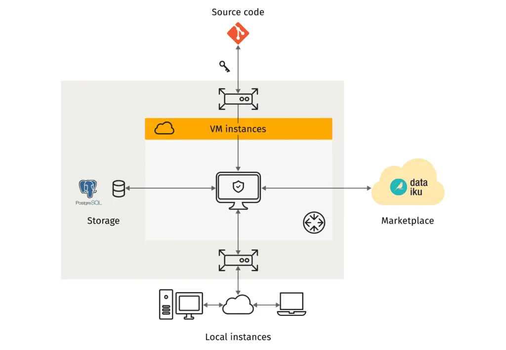
To implement the solution, we opted to utilize the Dataiku platform due to its practicality in bringing a product to market. Dataiku DSS is a powerful data science platform that enables users to build, test, and deploy machine learning models in an efficient way. Additionally, the inventory allocation optimization solution is compatible with their other products on the platform, such as the Demand Forecast component that may be used as an input generator for optimization purposes. In addition, the platform provides a wide range of tools for working with data, including visualization, data preparation, and machine learning algorithms.

For application hosting, we used cloud service VM instances with CentOS, which enables rapid deployment of pre-built images, while its future-proof approach allows scaling of analytical computation, as well as a convenient way to integrate real-time API-based models. It is also important to note that Dataiku is cloud-agnostic, and can be deployed to the majority of big cloud providers such as AWS, GCP and Azure.

As a last step, for the data storage, we used a PostgreSQL database from Cloud SQL GCP Service. Connecting Dataiku to the database was straightforward: we specified the database type, host, port, and other details in Dataiku DSS connection settings. More information about using SQL databases with Dataiku can be found here.

The figure below shows a schematic display of the high level architecture used for this implementation. The VM instance and PostgreSQL are within the same project in GCP, the Dataiku image is downloaded from the official website, and the implementation code for solving the mixed-integer programming problem is pulled from GridDynamics repo, which is integrated into the Dataiku DSS platform as a separate library.

Code implementation for the inventory allocation optimization solution is stored on GitHub, and the code itself is developed to support two different use cases; that is, as a python package or a script. In order to run a code on local setup as a script, you need to perform the following steps:

1. Pull code from git repository.
2. Install the local environment, by running the following command:

pipenv install -r requirements.txt

3. Change the files in the folder data with your files.

4. Check if the schema.yaml file reflects your current schema of data

5. Define the solver and mip_gap that you are going to use as  arguments values

6. Trigger the following function inside the source code:

python3 pipeline.py

For the implementation, we follow the builder design pattern to ensure the single responsibility principle, decoupled layers and re-usability. Therefore, future usage of the code enables easier scalability, adding functionalities and repurposing for implementations in more complex and/or similar problems to solve. By using the pattern, we implemented six separate utility modules, and they are:

1. data structure module for loading, formatting, and filtration of data/parameters;
2. module for variables that initialize decision variables;
3. constraint module that binds the optimization problem to predefined limitations;
4. objective function module that initializes the goal;
5. solver module for triggering the third-party MIP optimization problem; and finally
6. outputs module for retrieving and formatting the optimal solution as the output of the solver.

In addition, we have a notebooks directory in which we created the main notebook that is able to generate synthetic data, which can be used as part of the documentation for understanding the underlying structure, and relationship between data sources. Finally, we implemented configuration files in yaml format, so that users can change parameters of the run outside of the code, and conveniently version default parameters.

For third-party optimization software, we decided to implement OR-Tools by Google. OR-Tools is an open-source software suite for optimization, tuned for dealing with complicated problems such as integer, linear, mixed integer, and constraint programming. OR-Tools offers a Python API as well as other APIs for the most popular programming languages. In addition, OR-Tools supports a wide range of solvers: commercial solvers such as Gurobi and CPLEX, or open-source solvers such as SCIP, GLPK, GLOP, and CP-SAT. We use SCIP solver to tackle our mixed integer programming problem. Therefore, if additional capabilities are needed from the implemented solver, future users would not need to change a code implementation but just use the embedded plug&play mechanics of OR tools. This goes hand-in-hand with the main principle that we have in mind during code development, which is to decouple the functionality of the code.

In order to help users understand the relationship and process of generating data sources, we provide a notebook that could be used for various purposes such as: documentation, experimentation, or for generation of new synthetic data. The aim of this process is to portray a general structure that could be found in various industries that face similar inventory allocation optimization problems. Therefore, we generated the following list of datasets:

• warehouse_shipping_costs – information about shipping costs between warehouses and stores for individual product units;
• demand_nodes – list of product sets demand per demanding nodes;
• product_sets – contains information on mapping between product sets and product;
• warehouses – list of present warehouses, that is, supply nodes, with their respective capacity;  and
• warehouses_inventory – contains information about current product stock at different warehouses. Also contains information about the cost of procurement per product unit at different warehouses.

Generation of these datasets follows a logical order that maps relationships between data sources. Firstly, location of supply and demand nodes is generated by randomly selecting their physical location coordinates (in our example we generate nodes in the following three states: California, Nevada, and Arizona).

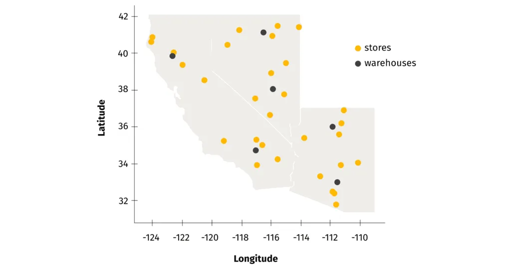
In parallel, we create a list of SKUs, their procurement costs, and the product sets to which they belong (product sets represent a basket/list of products that are regularly bought together, i.e. tomato sauce and pasta). In the following phase, we generate demand in each individual store by implementing poisson distribution for single product sets, while conserving demand sparsity (sparsity allows us to simulate the fact that not all product sets are significant or frequently represented in the population as individual SKUs).

As stated in the previous section, we model our problem in terms of product sets. In the setup, we have constraints that penalize split orders from different warehouses in order to avoid unnecessary shipping costs. Therefore, we group our products into product sets that represent products that are frequently bought together. Next, from the list of warehouses, we generate their capacity, and current on-hand quantity of SKUs. Finally, we generate the transportation cost of units between different warehouses and stores. For this, we use an approximation of driving distance between stores and warehouses. Therefore, shipping cost is the product between approximated distance and cost of unit per kilometer, which is constant.

At the end, the Dataiku solution itself implements an additional set of optional data sources, the usage of which depends on whether the optimization solutions are going to be compared with the benchmark or not. That is, if you would like to compare current optimal values with benchmark values, you need to provide an intended plan of inventory movement in the same format and schema as the output of the optimization pipeline. This is optional, and the whole solution can be run without benchmark data if you are only interested in optimal values. The list of optional datasets include:

• product_procurement_baseline – contains information about baseline procurement quantities for different warehouses.
• product_allocation_baseline – contains information about product quantities that were allocated from different warehouses to different stores.

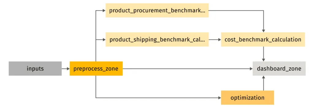
Since our project contains a fairly large amount of recipes and intermediate datasets in the flow, we use flow zones to organize them. All zones are tagged with specific colors. For instance, raw datasets are in the blue zone, the preprocessing zone is orange, the optimization zone is green, and the dashboard zone is red. A more detailed view of the Dataiku flow consists of seven zones:

• inputs – This zone consists of raw datasets described in the previous section. The input zone is connected to database tables that contain raw data. In our project, these datasets are synthetic. However, in customer use cases, datasets will be replaced with their own data. Moreover, this flow zone is compatible with an upstream service for demand forecasting, the output of which could be used as input.
• preprocess_zone – This zone is used for renaming columns to the format that is implemented internally in the code. Therefore, users are able to upload their data and choose column names in the application. After that, these column names are changed by the receipts in the preprocess_zone. This zone is mandatory and the output is raw datasets from inputs with renamed columns.
• product_procurement_benchmark_calculation – This is an optional zone when benchmark values are used. The purpose of it is to calculate benchmark procurement cost.
• product_shipping_benchmark_calculation – This is an optional zone when benchmark values are used. The purpose of it is to calculate the benchmark shipping cost.
• cost_benchmark_calculation – This is an optional zone. The input for this receipt are outputs from product_procurement_benchmark_calculation and product_shipping_benchmark_calculation zones. The output of these zones is the benchmark total cost.
• optimization – This zone is where the optimization procedure is run. It outputs the allocation of products across stores, procurement quantities in warehouses, stock quantities in warehouses, and optimal objective value. If we provide a benchmark as an input dataset, then the user is able to compare objective value with benchmark value.
• dashboard_zone – This zone is mandatory and contains recipes that prepare datasets for the dashboards.

Besides this, another technique for better flow organization and automation is to use scenarios. They come in handy when specific actions need to be performed as certain criteria are met. Therefore, scenarios are helpful in our use case because we have the option to compare baseline and new optimum values. Last but not least, we have an analytical dashboard that shows various data insights and optimization results. And in order for this to work flawlessly, we need at least one large scenario to run the entire flow in order to get all of these results.

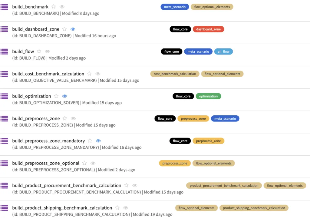
The illustration above provides information about implemented scenarios in the solution. As you can see, we used color coding with scenarios in a manner similar to the flow zones. The majority of our scenarios are step-based, with each step having its own receipt. Furthermore, we also have meta scenarios that execute other scenarios with corresponding tags. For actions connected to flows with baseline data, we have the tag flow optional elements.

In order to provide users with a convenient interface for implementing our solution, we apply Dataiku Application functionality. A packed Dataiku Project can be used as a visual interface to run recipes and scenarios in the project that can be shared with other users.

As a first step, the application provides an interface for establishing the connections with data storage. Dataiku supports different types of connections that can be used with our solution. Some of the more prominent ones are HDFS, Amazon S3, Azure Blob storage, Snowflake, Google Cloud Storage, and PostgreSQL.

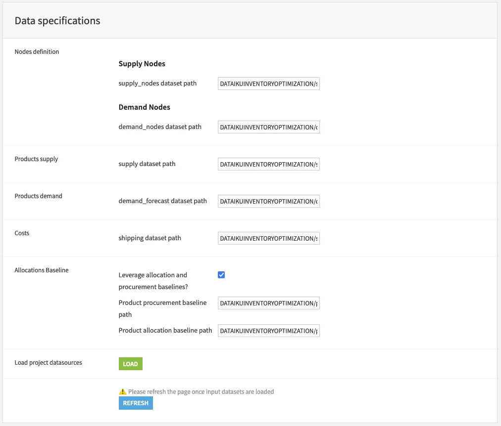
Next, the app executes a data specification step, which identifies all the necessary and optional datasets. In our case, it is used to specify table names from a PostgreSQL database that is connected with a Dataiku solution. Note that we have an optional Baseline checkbox, which is used to decide whether the new optimal values are going to be compared to the baseline metrics. If the baseline check box is selected, we can choose which data tables contain baseline information to be used for comparison in the later stages. There are also Optimization options which, if checked, display the results of the optimization in terms of product sets (item sets) rather than individual products.

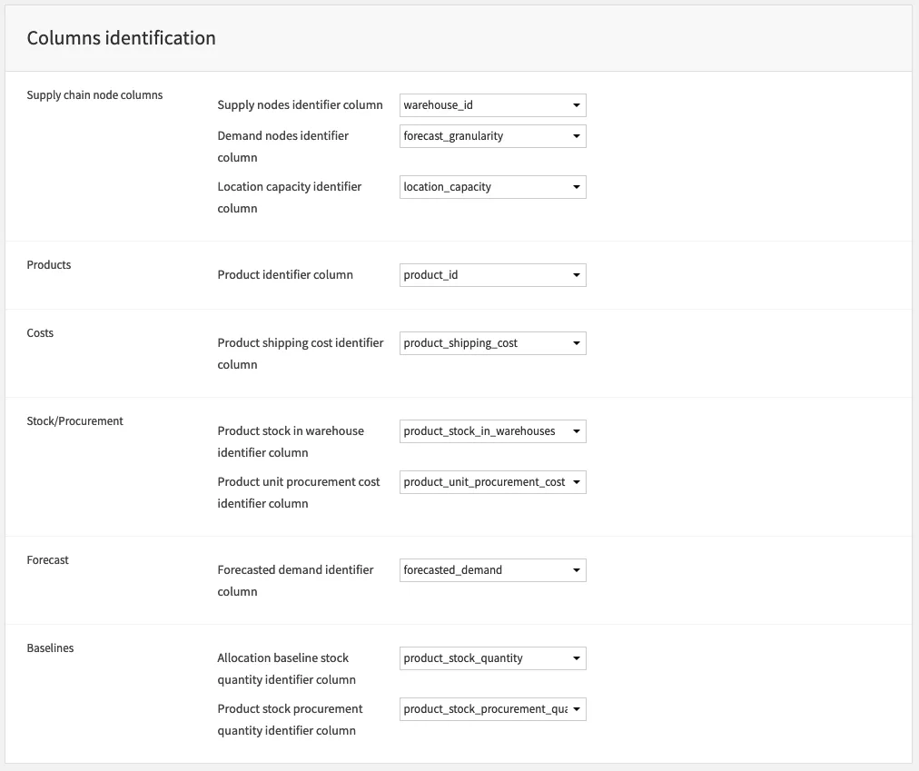
Following the data specifications step, you will move to the column identification step. With the tables having been specified in the previous step, the main goal here is to identify the relevant columns for the project. Essentially, we are mapping column names to the corresponding variables in the underlying code of the Dataiku scenarios. Note that the Baselines section is present here as well. The baselines field will be empty, however, if the baselines checkbox from the previous step was not selected. Moreover, the data specification step will have offered all the datasets that are present in the inputs flow zone as one of the options.

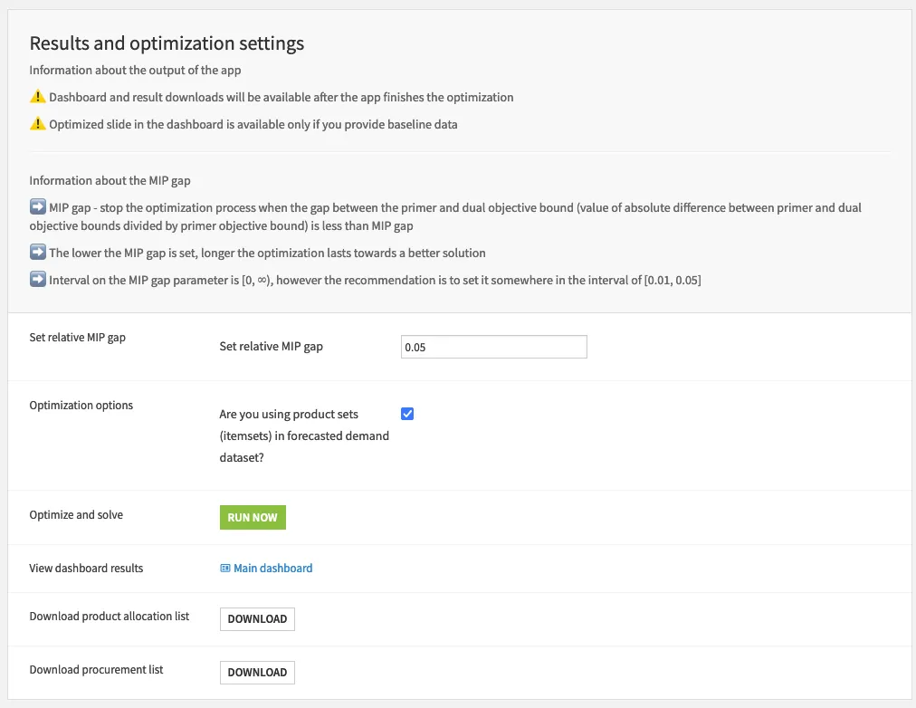
The final step in the pipeline is to tune the results and optimization settings. Here, the only choice is to specify the relative MIP gap. The MIP gap represents the tolerance value between the primer and dual objective bound (value of absolute difference between primer and dual objective bounds divided by primer objective bound). The lower the value,  the more optimal the solution we are going to get with higher value of execution time. Set the relative MIP gap tolerance, for instance, to 0.05 to tell the optimizer to stop as soon as it discovers a feasible integer solution that is within 5% of optimal. Finally, we run all required scenarios and update datasets for the dashboard zone by clicking the “Run Now” button.  After that, we can observe the insights in the custom dashboard, and download files with optimization results.

We developed the Dashboard section in the Dataiku solution for convenient visualization of insights from output datasets and optimization results. The goal is to provide relevant metrics for each part of the supply chain included in the inventory allocation optimization process. Therefore, we divided the dashboard into four main sections/tabs: Warehouse, Shipping, Procurement, and Benchmark.

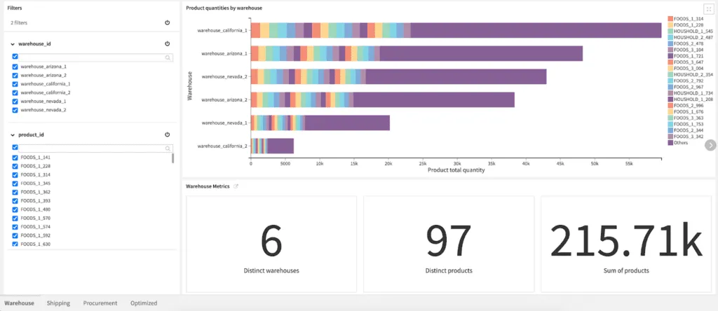
The capacity of various warehouses is compared in the Warehouse tab before and after optimization is submitted. The primary KPIs monitored are:

• the number of distinct products and warehouses;
• the total quantity of products that must be kept on hand; and
• the distribution of products among warehouses, displayed in pivot tables and bar plots.

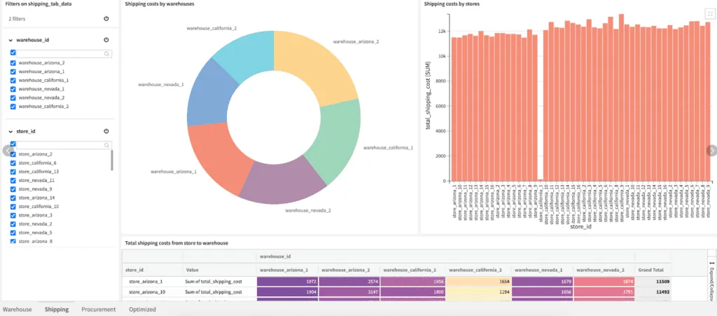
The Shipping tab gives more information about distribution of shipping costs per store, and shipping costs per warehouse. The primary KPIs that are monitored in this section are:

• total shipping cost;
• average shipping cost; and
• count of orders.

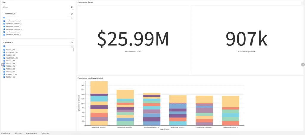
The Procurement tab displays the insights about procurement costs per warehouse and products. The primary KPIs that are monitored here are:

• procurement costs; and
• number of products to procure.

Finally, the Benchmark tab compares the optimized results with the benchmark results, showing the most important metrics related to procurement costs/quantities and shipping costs/quantities. The main KPIs that are tracked in this section are:

• optimized vs old cost;
• baseline vs optimal product stock quantity;
• baseline vs optimized procurement costs;
• baseline vs optimized product quantity; and
• baseline vs optimized shipping cost.

All the dashboards have filters for selecting all or a group of warehouses, while some tabs have additional filters for stores and products. All the data displayed in the Dashboard section were prepared inside the Dashboard flow zone.

The first and most important step on the supply chain management journey for any business should be inventory optimization. When inventory is optimally allocated, cost efficiency, productivity, and customer satisfaction are all significantly improved.

In this blog post, we’ve shown how you can make more informed inventory level decisions to meet customer demands and cut costs by carefully considering a variety of factors, including demand forecasting, procurement, order splitting, and shipping costs with a single solution: The Inventory Allocation Optimization Starter Kit.

The solution can be extended with various features such as procurement shipping capacity constraints, region-level constraints, and more. The created pipeline can also be transformed into a replenishment control solution that optimizes not only the static inventory allocation levels, but also replenishment and shipping times.

Ready to optimize your supply chain and inventory management? Get in touch with us to start a conversation.